Harmonic
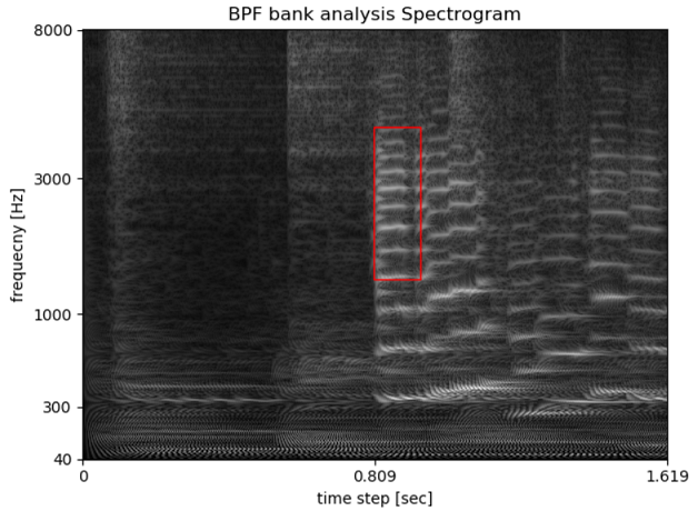
BPF bank analysis Spectrogram
Spectrogram analysis of Tube Amplifier Distortion (PC simulation)
feature
- BPF’s target response is 2nd harmonic level less than -70dB
- Mel-frequency division
- Half-wave rectification until a few KHz signal or DC with ripple signal
- Down sampling to decrease temporal resolution
- N-th root compression
description
- BPF_analysis1.py BPF bank analysis Spectrogram main program
- BPF4.py IIR Band Pass Filter, process twice. Target response is 2nd harmonic level less than -70dB
- Compressor1.py compressor by power(input,1/3.5), 3.5 root compression
- ema1.py Exponential Moving Average with Half-wave rectification, and smoothing via lpf
- iir1.py iir butterworth filter
- mel.py mel-frequency equal shifted list
- compare_spectrograms1.py main program, compare matching portion of two spectrograms and show its difference
- search_similar_area1.py main program, search some similar area near the specified area in spectrogram
- Spectrogram_2D-FFT.py main program, show Spectrogram, 2D inverse FFT, and 2D FFT of the spectrogram
- stereo_channel_matching.py main program, search some similar area to the specified area in another channel spectrogram
- in the wav folder, there are used wav files.
analysis of Tube Amplifier Distortion (PC simulation)
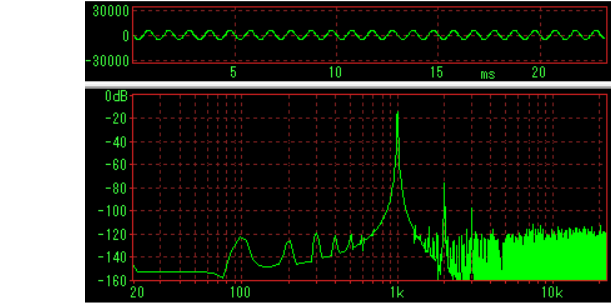
Input signal is 1KHz -10dB sin wave
FFT spectrum of 1KHz-10dB_44100Hz_400ms-TwoTube_stereo.wav. There are 2nd harmonic(2KHz) and 3rd harmonic(3KHz).
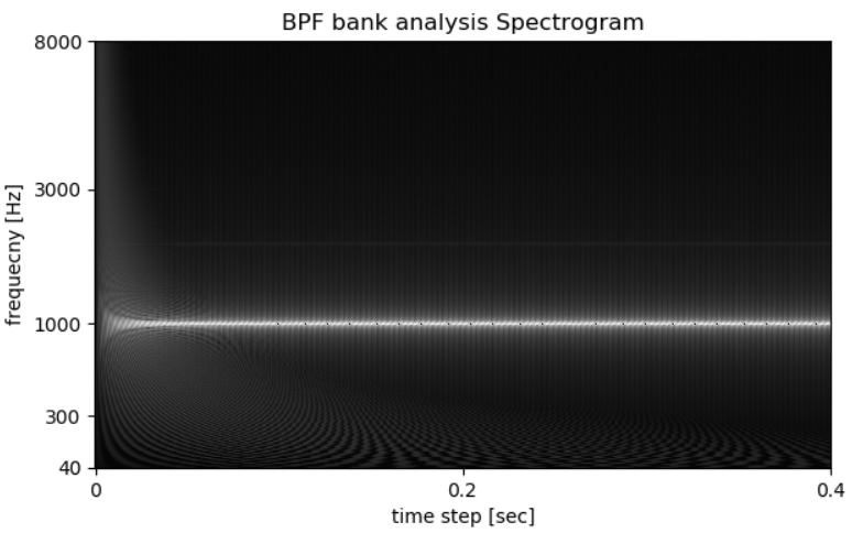
BPF_analysis1.py output. Dark white line in the mid area shows 2nd harmonic(2KHz). Bright white line shows 1KHz.
Start wave pattern is filter transient response.
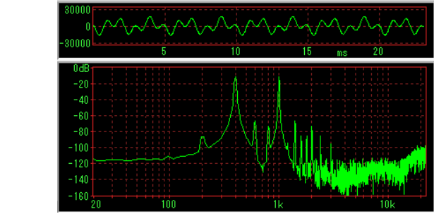
Input signal is mix of 400Hz -10dB sin wave and 1KHz -10dB sin wave
FFT spectrum of Mix_400Hz1KHz-10dB_44100Hz_400msec_TwoTube_mono.wav. There are 600Hz, 1400Hz, etc other than 800Hz, 2KHz, 1600Hz and 3000Hz.
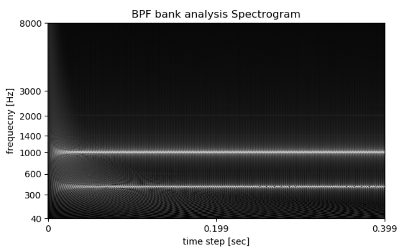
BPF_analysis1.py output. Dark white lines show 600Hz, 1400Hz, and 2KHz.
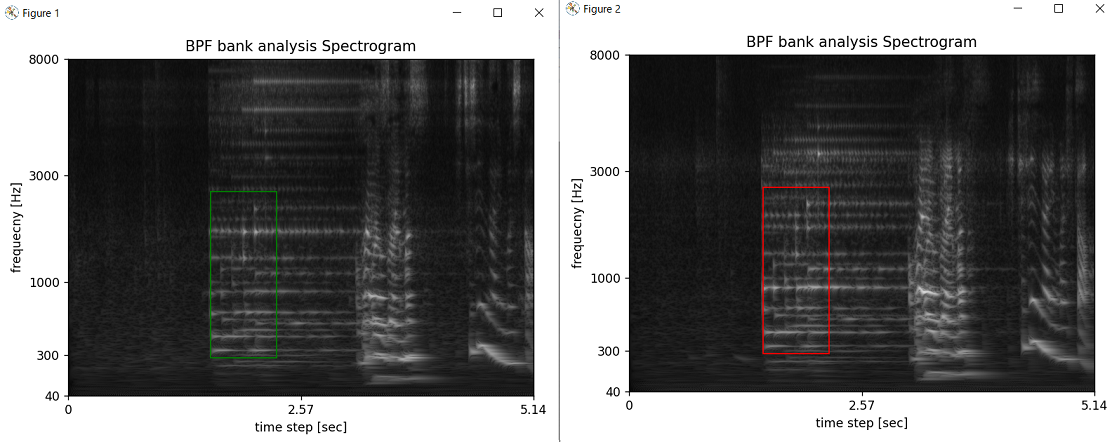
Compare matching portion of two spectrograms
A music spectrogram comparison of input and output of Tube Amplifier (PC simulation).
Matching portion (red rectangle area) in the template spectrogram to compare.
Set diagonal position by pointing-device mouse and exist figure. Matching portion in the matching spectrogram will be detected by cv2.matchTemplate function.
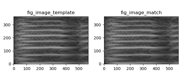
each matching portion of template spectrogram and matching spectrogram
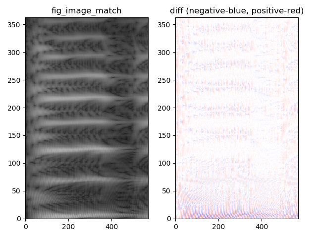
matching portion and its difference (red means positive and blue means negative)
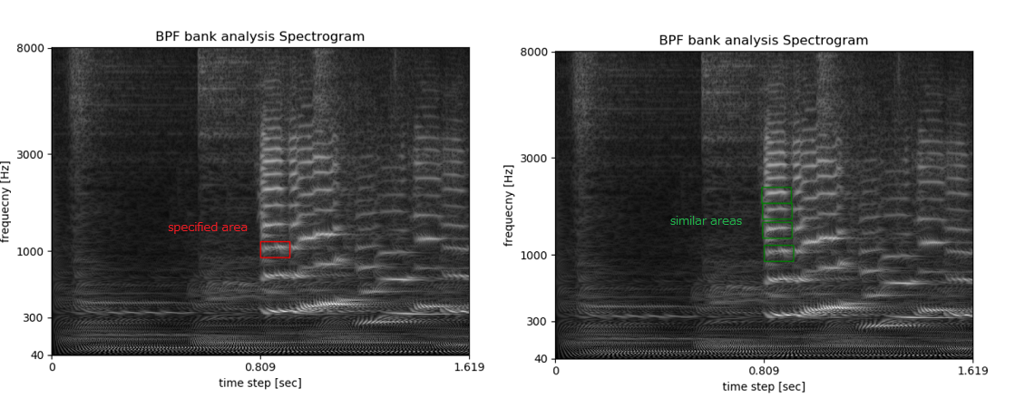
Search some similar area near the specified area in spectrogram
Specify the area as diagonal position by pointing-device mouse. And then, click right mouse button or press m on keyboard.
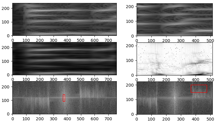
Spectrogram, 2D FFT, and 2D inverse FFT
In the following figure, from top to bottom, spectrogram, 2D inverse FFT of red rectangle in 2D FFT, and 2D FFT of the spectrogram.
Search some similar area to the specified area in another channel spectrogram
Load stero(2 channel) wav file and make Spectrogram per each channel (show Figure 1 and Figure 2).
Search some similar area to the specified area in another channel.
Specify the area as diagonal position by pointing-device mouse. And then, click right mouse button or press m on keyboard.
After above completed, then press c on keyboard. It will compute difference between both channel, after time correction.
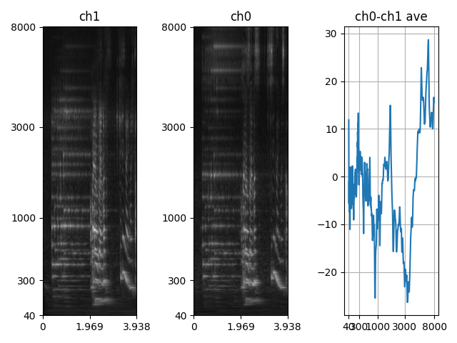
Peak or bottom in the difference, frequency characteristic between channels, is significant, because real signal is available at the point to be compared.
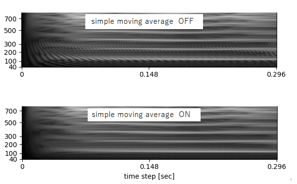
Accentuate ridge of local peak in lower frequency
BPF_analysis2.py was added simple moving average until 800Hz signal to accentuate ridge of local peak.
License
MIT
Regarding to nms.py, please refer copyright and license notice in the content.